SEXS-PTI

Simplified excitation-system model.

Block Diagram

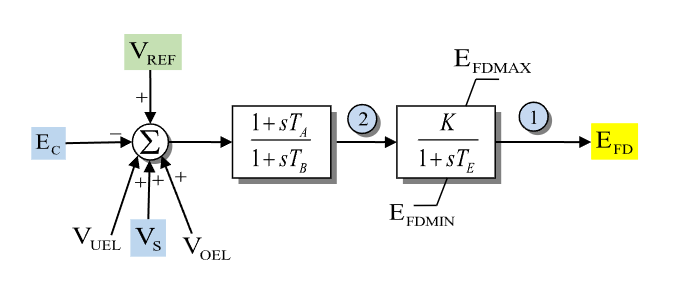
Figure 1: Exciter SEXS-PTI model. Figure courtesy of PowerWorld

Model Parameters

Symbol	Units	JSON	Description	Typical Value	Note
\(T_A\)	[s]	Ta	Numerator time constant of lead–lag block
\(T_B\)	[s]	Tb	Denominator time constant of lead–lag block
\(T_E\)	[s]	Te	Exciter field time constant
\(K\)	[p.u.]	K	Voltage regulator gain
\(E_{\mathrm{fd}}^{\max}\)	[p.u.]	Efdmax	Maximum excitation output
\(E_{\mathrm{fd}}^{\min}\)	[p.u.]	Efdmin	Minimum excitation output

PowerWorld/PSS/E SEXS_PTI data often gives \(T_A/T_B\) as a ratio. GridKit stores \(T_A\) and \(T_B\) separately, so convert ratio-format data with \(T_A = (T_A/T_B)T_B\) before passing parameters to the model.

All six parameters are required; there are no defaults.

Parameter Validation

A valid SEXS-PTI parameter set must satisfy the following conditions:

\[\begin{split}\begin{aligned} T_A &\ge 0 \\ T_B, T_E, K &> 0 \\ E_{\mathrm{fd}}^{\min} &< E_{\mathrm{fd}}^{\max} \end{aligned}\end{split}\]

Model Derived Parameters

None.

Model Ports

Name	Port	Init	Description
bus	Bus	Known	Terminal bus voltage
vref	Input	Unknown	Voltage-control reference
vs	Input	Known	Stabilizer input signal
vuel	Input	Known	Under-excitation limiter input
voel	Input	Known	Over-excitation limiter input
efd	Output	Known	Required field-voltage output seeded by the machine

Model Variables

Internal Variables

Differential

Symbol	Units	Description	Note
\(V_R\)	[p.u.]	Lead–lag block state
\(E_{\mathrm{fd}}\)	[p.u.]	Exciter field voltage output

Algebraic

Symbol	Units	Description	Note
\(V_{\mathrm{tr}}\)	[p.u.]	Terminal voltage error signal

External Variables

Differential

None.

Algebraic

Symbol	Units	Description	Note
\(V_r\)	[p.u.]	Terminal voltage, real component	Bus input
\(V_i\)	[p.u.]	Terminal voltage, imaginary component	Bus input
\(V_{\mathrm{ref}}\)	[p.u.]	Reference voltage	Signal port vref
\(V_S\)	[p.u.]	Stabilizer output	Signal port vs
\(V_{\mathrm{oel}}\)	[p.u.]	Over-excitation limiter signal	Signal port voel
\(V_{\mathrm{uel}}\)	[p.u.]	Under-excitation limiter signal	Signal port vuel

Model Equations

Smooth functions: antiwindup.

\[E_C = \sqrt{V_r^2+V_i^2}\]

Internal Equations

Differential

\[\begin{split}\begin{aligned} f &= \dfrac{-E_{\mathrm{fd}}+(K/T_B)(-V_R+T_AV_{\mathrm{tr}})}{T_E} \\ 0 &= -\dot V_R-V_{\mathrm{tr}}+\dfrac{-V_R+T_AV_{\mathrm{tr}}}{T_B} \\ 0 &= -\dot E_{\mathrm{fd}}+\text{antiwindup}(E_{\mathrm{fd}},f;E_{\mathrm{fd}}^{\min},E_{\mathrm{fd}}^{\max}) \end{aligned}\end{split}\]

Algebraic

\[\begin{aligned} 0&=-V_{\mathrm{tr}}-E_C+V_{\mathrm{ref}}+V_S+V_{\mathrm{oel}}+V_{\mathrm{uel}} \end{aligned}\]

External Equations

None.

Initialization

The generator initializes the EFD signal first. SEXS-PTI then reads that value and any attached \(V_S\), \(V_{\mathrm{oel}}\), and \(V_{\mathrm{uel}}\) signals and assumes steady state:

\[\begin{split}\begin{aligned} V_{\mathrm{tr}} &\leftarrow \dfrac{E_{\mathrm{fd}}}{K} \\ V_R &\leftarrow (T_A - T_B)V_{\mathrm{tr}} \\ V_{\mathrm{ref}} &\leftarrow E_C + V_{\mathrm{tr}} - V_S - V_{\mathrm{oel}} - V_{\mathrm{uel}} \end{aligned}\end{split}\]

All derivatives initialize to zero.

Monitors

Monitor	Units	Description	Note
efd	[p.u.]	Field-voltage output	\(E_{\mathrm{fd}}\)