EXAC2

EXAC2 is an IEEE Type AC excitation system with a voltage transducer, lead–lag input compensation, limited voltage-amplifier state, low-value gate, voltage regulator limits, exciter alternator state, stabilizing feedback, rectifier loading, saturation, and optional speed multiplier.

Warning

Initialization does not yet invert the smooth gates and limits used by the model equations.

Notes

• Internal voltage and current signals are on model base unless otherwise stated.

• The rectifier loading block \(F_{\mathrm{ex}}=f(I_N)\) is the source AC-exciter loading curve from Fig. 1; it is not a CommonMath helper.

• The source diagram labels the optional multiplier input as Speed; GridKit uses machine speed deviation, so the enabled multiplier is \(1+\omega\).

Block Diagram

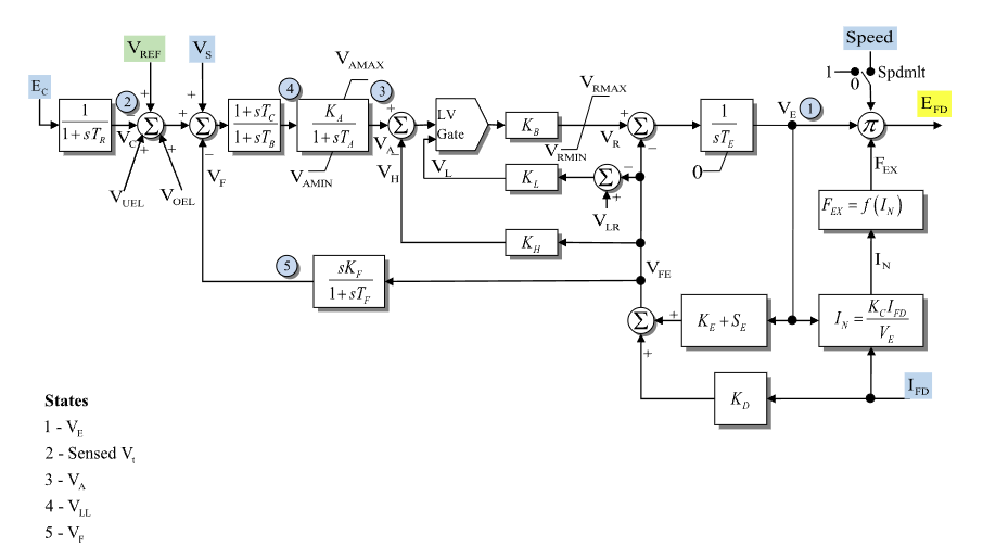
Figure 1: Exciter EXAC2 model. Figure courtesy of PowerWorld

Model Parameters

Symbol	Units	JSON	Description	Typical Value	Note
\(T_R\)	[s]	Tr	Transducer time constant	0.0	if zero, \(V_C\) is algebraic
\(T_B\)	[s]	Tb	Lag time constant for voltage-regulator input lead–lag	0.0
\(T_C\)	[s]	Tc	Lead time constant for voltage-regulator input lead–lag	0.0
\(K_A\)	[p.u.]	Ka	Voltage-amplifier gain	40.0
\(T_A\)	[s]	Ta	Voltage-amplifier time constant	0.1
\(V_A^{\max}\)	[p.u.]	VaMax	Maximum voltage-amplifier output	1.0	Source label: VAMAX
\(V_A^{\min}\)	[p.u.]	VaMin	Minimum voltage-amplifier output	-1.0	Source label: VAMIN
\(K_B\)	[p.u.]	Kb	Regulator pre-limit gain after low-value gate	1.0	Source label: KB
\(V_R^{\max}\)	[p.u.]	Vrmax	Maximum voltage-regulator output	1.0
\(V_R^{\min}\)	[p.u.]	Vrmin	Minimum voltage-regulator output	-1.0
\(T_E\)	[s]	Te	Exciter alternator time constant	0.5
\(K_L\)	[p.u.]	Kl	Field-current limiter feedback gain	0.0	Source label: KL
\(K_H\)	[p.u.]	Kh	Regulator feedback path gain	0.0	Source label: KH
\(K_F\)	[p.u.]	Kf	Stabilizing feedback gain	0.05
\(T_F\)	[s]	Tf	Stabilizing feedback time constant	0.7	if zero, \(V_F\) is algebraic
\(K_C\)	[p.u.]	Kc	Rectifier loading current coefficient	0.0	forms \(I_N\)
\(K_D\)	[p.u.]	Kd	Demagnetizing factor feedback gain	0.0
\(K_E\)	[p.u.]	Ke	Exciter field-resistance line-slope margin	0.1
\(V_{\mathrm{lr}}\)	[p.u.]	VLr	Low-value gate lower reference	0.0	Source label: VLR
\(E_1\)	[p.u.]	E1	First saturation voltage point	2.8
\(S_E(E_1)\)	[p.u.]	SE1	Saturation value at \(E_1\)	0.08	Source label: Se1
\(E_2\)	[p.u.]	E2	Second saturation voltage point	3.7
\(S_E(E_2)\)	[p.u.]	SE2	Saturation value at \(E_2\)	0.33	Source label: Se2
\(s_{\mathrm{spd}}\)	[binary]	Spdmlt	Speed multiplier flag	0	1 enables the speed multiplier

Parameter Validation

A valid EXAC2 parameter set must satisfy the following conditions:

\[\begin{split}\begin{aligned} &K_A > 0 \\ &T_R \ge 0,\quad T_A > 0,\quad T_B \ge 0,\quad T_C \ge 0,\quad T_E > 0,\quad T_F \ge 0 \\ &T_B > 0\quad\text{or}\quad(T_B = 0\ \text{and}\ T_C = 0) \\ &V_A^{\min} \le V_A^{\max},\quad V_R^{\min} \le V_R^{\max} \\ &s_{\mathrm{spd}} \in \{0,1\} \end{aligned}\end{split}\]

The saturation points follow the same two-point validation used by other exciter READMEs: both saturation values are zero, or both points define a valid positive quadratic fit.

Model Derived Parameters

The saturation curve is fitted from the two supplied saturation points. If both saturation factors are zero, use \(S_A=0\) and \(S_B=0\). Otherwise:

\[\begin{split}\begin{aligned} C &= \sqrt{\dfrac{S_E(E_2)}{S_E(E_1)}} \\ S_A &= \dfrac{C E_1 - E_2}{C - 1} \\ S_B &= \dfrac{S_E(E_1)}{(E_1 - S_A)^2} \end{aligned}\end{split}\]

Model Ports

Name	Port	Init	Description
ec	Input	TBD	Compensated terminal voltage magnitude \(E_C\)
vref	Input	TBD	Voltage-control reference \(V_{\mathrm{ref}}\)
vs	Input	TBD	Stabilizer input signal \(V_S\)
vuel	Input	TBD	Under-excitation limiter input \(V_{\mathrm{uel}}\)
voel	Input	TBD	Over-excitation limiter input \(V_{\mathrm{oel}}\)
ifd	Input	TBD	Machine field current \(I_{\mathrm{fd}}\)
speed	Input	TBD	Machine speed deviation \(\omega\)
efd	Output	TBD	Field-voltage output \(E_{\mathrm{fd}}\)

Model Variables

Internal Variables

Differential

Symbol	Units	Description	Note
\(V_E\)	[p.u.]	Exciter alternator voltage state before output multipliers	State 1 in Fig. 1; Source label: VE
\(V_C\)	[p.u.]	Sensed compensated voltage	State 2 in Fig. 1; Source label: Sensed Vt; algebraic when \(T_R=0\)
\(V_A\)	[p.u.]	Limited voltage-amplifier output	State 3 in Fig. 1; Source label: VA
\(x_{\mathrm{LL}}\)	[p.u.]	Lead–lag block state	State 4 in Fig. 1; Source label: VLL
\(V_F\)	[p.u.]	Stabilizing feedback washout output	State 5 in Fig. 1; Source label: VF; algebraic when \(T_F=0\)

Algebraic

Symbol	Units	Description	Note
\(e_V\)	[p.u.]	Voltage-regulator input error before lead–lag block	Summing junction after sensed voltage
\(V_{\mathrm{LL}}\)	[p.u.]	Lead–lag output	Input to voltage amplifier
\(V_H\)	[p.u.]	Regulator feedback path signal	Source label: KH
\(V_L\)	[p.u.]	Field-current limiter low-value gate input	Source label: KL; lower reference \(V_{\mathrm{lr}}\)
\(V_{\mathrm{lv}}\)	[p.u.]	Low-value gate output	Lesser of amplifier path and limiter path
\(V_R\)	[p.u.]	Voltage-regulator output	Limited by \(V_R^{\min}\) and \(V_R^{\max}\)
\(S_E\)	[p.u.]	Saturation coefficient evaluated at \(V_E\)	Uses derived saturation curve
\(I_N\)	[p.u.]	Normalized exciter loading current	Source label: IN; satisfies \(V_E I_N=K_C I_{\mathrm{fd}}\)
\(F_{\mathrm{ex}}\)	[p.u.]	Rectifier loading factor	Source label: FEX; source curve \(F_{\mathrm{ex}}=f(I_N)\)
\(V_{\mathrm{FE}}\)	[p.u.]	Exciter feedback signal	Sum of saturation/resistance and \(K_D I_{\mathrm{fd}}\) paths
\(E_{\mathrm{fd}}\)	[p.u.]	Field-voltage output	Output after rectifier loading and optional speed multiplier

External Variables

Differential

None.

Algebraic

Symbol	Units	Description	Note
\(E_C\)	[p.u.]	Compensated terminal voltage magnitude	Source label: EC
\(V_{\mathrm{ref}}\)	[p.u.]	Voltage-control reference	Source label: VREF
\(V_S\)	[p.u.]	Stabilizer input signal	Source label: VS; optional, defaults to zero
\(V_{\mathrm{uel}}\)	[p.u.]	Under-excitation limiter input	Source label: VUEL; optional, defaults to zero
\(V_{\mathrm{oel}}\)	[p.u.]	Over-excitation limiter input	Source label: VOEL; optional, defaults to zero
\(I_{\mathrm{fd}}\)	[p.u.]	Machine field current	Source label: IFD
\(\omega\)	[p.u.]	Machine speed deviation	Source label: Speed; optional when \(s_{\mathrm{spd}}=0\)

Model Equations

Smooth functions: antiwindup, clamp, min, \(q\).

Internal Equations

Differential

\[\begin{split}\begin{aligned} 0 &= -T_R\dot V_C - V_C + E_C \\ 0 &= -T_B\dot x_{\mathrm{LL}} - x_{\mathrm{LL}} + e_V \\ 0 &= -T_A\dot V_A + \text{antiwindup}\!( V_A, -V_A + K_A V_{\mathrm{LL}}; V_A^{\min}, V_A^{\max} ) \\ 0 &= -T_E\dot V_E + V_R - V_{\mathrm{FE}} \\ 0 &= -T_F\dot V_F - V_F + K_F\dot V_E \end{aligned}\end{split}\]

Algebraic

\[\begin{split}\begin{aligned} 0 &= -e_V + V_{\mathrm{ref}} + V_S + V_{\mathrm{uel}} + V_{\mathrm{oel}} - V_C - V_F \\ 0 &= -T_B(V_{\mathrm{LL}} - x_{\mathrm{LL}}) + T_C(e_V - x_{\mathrm{LL}}) \\ 0 &= -V_H + K_H V_{\mathrm{FE}} \\ 0 &= -V_L + V_{\mathrm{lr}} + K_L V_{\mathrm{FE}} \\ 0 &= -V_{\mathrm{lv}} + \text{min}(V_A + V_H,\ V_L) \\ 0 &= -V_R + \text{clamp}(K_B V_{\mathrm{lv}}; V_R^{\min}, V_R^{\max}) \\ 0 &= -S_E + S_B\,q(V_E - S_A) \\ 0 &= -V_E I_N + K_C I_{\mathrm{fd}} \\ 0 &= -F_{\mathrm{ex}} + f(I_N) \\ 0 &= -V_{\mathrm{FE}} + (K_E + S_E)V_E + K_D I_{\mathrm{fd}} \\ 0 &= -E_{\mathrm{fd}} + (1+s_{\mathrm{spd}}\omega)F_{\mathrm{ex}}V_E \end{aligned}\end{split}\]

When \(T_B=T_C=0\), the lead–lag block is bypassed so \(V_{\mathrm{LL}}=e_V\).

External Equations

None.

Initialization

The machine initializes \(E_{\mathrm{fd}}\) and \(I_{\mathrm{fd}}\) first. For a standard unsaturated start, EXAC2 reads those values, sets all internal derivatives to zero, and first solves the coupled rectifier-loading equations:

\[\begin{split}\begin{aligned} 0 &= -V_E I_N + K_C I_{\mathrm{fd}} \\ 0 &= -F_{\mathrm{ex}} + f(I_N) \\ 0 &= -E_{\mathrm{fd}} + (1+s_{\mathrm{spd}}\omega)F_{\mathrm{ex}}V_E \end{aligned}\end{split}\]

Then evaluate the feedback path:

\[\begin{split}\begin{aligned} S_E &\leftarrow S_B\,q(V_E - S_A) \\ V_{\mathrm{FE}} &\leftarrow (K_E + S_E)V_E + K_D I_{\mathrm{fd}} \end{aligned}\end{split}\]

Then solve the low-value gate and voltage-regulator chain:

\[\begin{split}\begin{aligned} V_R &\leftarrow V_{\mathrm{FE}} \\ V_H &\leftarrow K_H V_{\mathrm{FE}} \\ V_L &\leftarrow V_{\mathrm{lr}} + K_L V_{\mathrm{FE}} \\ V_{\mathrm{lv}} &\leftarrow \dfrac{V_R}{K_B} \\ V_A &\leftarrow V_{\mathrm{lv}} - V_H \\ V_{\mathrm{LL}} &\leftarrow \dfrac{V_A}{K_A} \\ V_C &\leftarrow E_C \\ V_F &\leftarrow 0 \\ e_V &\leftarrow V_{\mathrm{LL}} \\ x_{\mathrm{LL}} &\leftarrow e_V \\ V_{\mathrm{ref}} &\leftarrow e_V + V_C + V_F - V_S - V_{\mathrm{uel}} - V_{\mathrm{oel}} \end{aligned}\end{split}\]

This standard start requires \(1+s_{\mathrm{spd}}\omega\ne 0\), \(V_E\ne 0\), \(K_A\ne 0\), \(K_B\ne 0\), inactive \(V_A\) and \(V_R\) limits, and the low-value gate selecting the amplifier path. Starts with active low-value gate limiting or saturated regulator states are outside these closed-form equations.

Monitors

Monitor	Units	Description	Note
efd	[p.u.]	Field-voltage output	\(E_{\mathrm{fd}}\)
ve	[p.u.]	Exciter alternator voltage state	\(V_E\)
vc	[p.u.]	Sensed compensated voltage	\(V_C\)
va	[p.u.]	Voltage-amplifier state	\(V_A\)
vr	[p.u.]	Voltage-regulator output	\(V_R\)
vll	[p.u.]	Lead–lag output	\(V_{\mathrm{LL}}\)
vf	[p.u.]	Stabilizing feedback state	\(V_F\)
vlv	[p.u.]	Low-value gate output	\(V_{\mathrm{lv}}\)
in	[p.u.]	Normalized exciter loading current	\(I_N\)
fex	[p.u.]	Rectifier loading factor	\(F_{\mathrm{ex}}\)
se	[p.u.]	Saturation coefficient	\(S_E\)