Branch

The Branch model represents a two-terminal phasor-domain \(\pi\) branch with an optional off-nominal tap magnitude and phase shift on bus 1. Terminal current contributions are oriented entering the adjacent buses.

Notes

• Setting \(\tau = 1\) and \(\theta = 0\) gives the ordinary symmetric transmission-line \(\pi\) model.

• The total line shunt \(G + jB\) is split equally between the two terminals, while the magnetizing shunt \(G_\mathrm{mag} + jB_\mathrm{mag}\) is connected at bus 1; both shunts are added outside the \(\mathbf{M}\) transformation.

• The branch has no solver-owned variables; it contributes current residuals directly to the connected buses.

• Taking a branch out of service can make the system Jacobian singular, which the model does not detect. See Appendix A and Appendix B.

Block Diagram

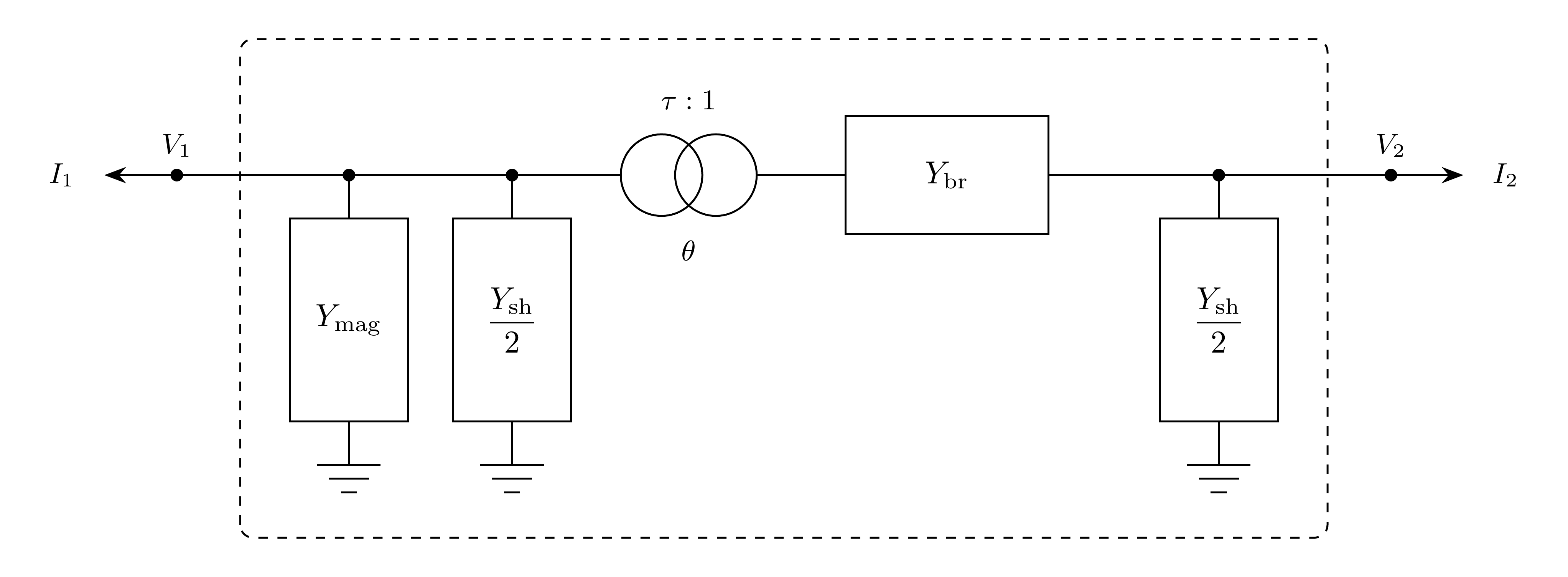
Figure 1: Branch model.

Model Parameters

Symbol	Units	JSON	Description	Typical Value	Note
\(R\)	[p.u.]	R	Branch series resistance
\(X\)	[p.u.]	X	Branch series reactance	0.01	Default when omitted
\(G\)	[p.u.]	G	Total line shunt conductance	0.0
\(B\)	[p.u.]	B	Total line shunt susceptance	0.0
\(G_\mathrm{mag}\)	[p.u.]	Gmag	Magnetizing shunt conductance at bus 1	0.0
\(B_\mathrm{mag}\)	[p.u.]	Bmag	Magnetizing shunt susceptance at bus 1	0.0
\(\tau\)	[p.u.]	tap	Off-nominal tap magnitude on bus-1 side	1.0
\(\theta\)	[rad]	phase	Phase-shift angle	0.0

Parameter Validation

A valid Branch parameter set must satisfy the following conditions:

\[\begin{split}\begin{aligned} &R, X, G, B, G_\mathrm{mag}, B_\mathrm{mag}, \tau, \theta \in \mathbb{R}\ \text{and finite} \\ &R^2 + X^2 > 0 \\ &\tau > 0 \end{aligned}\end{split}\]

Model Derived Parameters

The series, magnetizing shunt, and line shunt admittances are:

\[\begin{split}\begin{aligned} Y_{\mathrm{br}} &= \dfrac{1}{R + jX} \\ Y_{\mathrm{mag}} &= G_\mathrm{mag} + jB_\mathrm{mag} \\ Y_{\mathrm{sh}} &= G + jB \end{aligned}\end{split}\]

The series, magnetizing shunt, and line shunt admittance matrices are:

\[\begin{split}\begin{aligned} \mathbf{Y}_0 &= \begin{bmatrix} -Y_{\mathrm{br}} & Y_{\mathrm{br}} \\ Y_{\mathrm{br}} & -Y_{\mathrm{br}} \end{bmatrix} \\ \mathbf{Y}_\mathrm{mag} &= \begin{bmatrix} -Y_{\mathrm{mag}} & 0 \\ 0 & 0 \end{bmatrix} \\ \mathbf{Y}_\mathrm{sh} &= \dfrac{1}{2} \begin{bmatrix} -Y_{\mathrm{sh}} & 0 \\ 0 & -Y_{\mathrm{sh}} \end{bmatrix} \end{aligned}\end{split}\]

The off-nominal transformer transformation uses bus 1 as the tap side:

\[\begin{split}\begin{aligned} \mathbf{M} &= \begin{bmatrix} \tau^{-1} & 0 \\ 0 & \exp(j\theta) \end{bmatrix} \end{aligned}\end{split}\]

The magnetizing and line shunts are added outside the transformation, and the service status \(u\) scales the whole branch:

\[\begin{aligned} \mathbf{Y} &= u \left( \mathbf{M}^{\dagger} \mathbf{Y}_0 \mathbf{M} + \mathbf{Y}_\mathrm{mag} + \mathbf{Y}_\mathrm{sh} \right) \end{aligned}\]

For the equations below, write each entry as \(Y_{mn}=G_{mn}+jB_{mn}\).

Model Ports

Name	Port	Init	Description
bus1	Bus	Known	Required bus-1 terminal; the tapped side
bus2	Bus	Known	Required bus-2 terminal

Model Variables

Internal Variables

Differential

None.

Algebraic

None.

External Variables

Differential

None.

Algebraic

Symbol	Units	Description	Note
\(V_{r1}\)	[p.u.]	Terminal voltage, real component, bus 1	Owned by bus object
\(V_{i1}\)	[p.u.]	Terminal voltage, imaginary component, bus 1	Owned by bus object
\(V_{r2}\)	[p.u.]	Terminal voltage, real component, bus 2	Owned by bus object
\(V_{i2}\)	[p.u.]	Terminal voltage, imaginary component, bus 2	Owned by bus object

Model Equations

Internal Equations

Differential

None.

Algebraic

None.

External Equations

The branch current relation is \(0 = -\mathbf{I} + \mathbf{Y}\mathbf{V}\).

\[\begin{split}\begin{aligned} I_{r1} &= G_{11} V_{r1} - B_{11} V_{i1} + G_{12} V_{r2} - B_{12} V_{i2} \\ I_{i1} &= B_{11} V_{r1} + G_{11} V_{i1} + B_{12} V_{r2} + G_{12} V_{i2} \\ I_{r2} &= G_{21} V_{r1} - B_{21} V_{i1} + G_{22} V_{r2} - B_{22} V_{i2} \\ I_{i2} &= B_{21} V_{r1} + G_{21} V_{i1} + B_{22} V_{r2} + G_{22} V_{i2} \end{aligned}\end{split}\]

These current contributions are added to the connected bus residuals with positive sign because branch current is oriented entering the bus.

Initialization

The Branch model has no internal state to initialize. During construction or parameter updates, the component computes \(\mathbf{Y}\) from the current parameter values. Terminal current and power monitor values are evaluated from the connected bus voltages when read. Parameter verification enforces the conditions in Parameter Validation.

Monitors

Monitor	Units	Description	Note
ir1	[p.u.]	Terminal current, real component, bus 1	Oriented entering bus 1
ii1	[p.u.]	Terminal current, imaginary component, bus 1	Oriented entering bus 1
im1	[p.u.]	Terminal current magnitude, bus 1
p1	[p.u.]	Active power at bus 1 terminal	Positive entering bus 1
q1	[p.u.]	Reactive power at bus 1 terminal	Positive entering bus 1
ir2	[p.u.]	Terminal current, real component, bus 2	Oriented entering bus 2
ii2	[p.u.]	Terminal current, imaginary component, bus 2	Oriented entering bus 2
im2	[p.u.]	Terminal current magnitude, bus 2
p2	[p.u.]	Active power at bus 2 terminal	Positive entering bus 2
q2	[p.u.]	Reactive power at bus 2 terminal	Positive entering bus 2

Appendix A: Out-of-Service Branches

Taking a branch out of service changes the system Jacobian and can make it singular. Let the system be described by the DAE \(\mathbf{F}(\mathbf{x}, \dot{\mathbf{x}}, t) = \mathbf{0}\). For a purely algebraic network, \(\mathbf{x} = \mathbf{V}\) are the bus voltages and

\[\mathbf{F}(\mathbf{V}) = -\mathbf{I} + \mathbf{Y}\mathbf{V}\]

where \(\mathbf{I}\) is the current injected by devices and \(\mathbf{Y}\) is the bus admittance matrix. In the three-bus example below, bus 1 has a Norton generator, a constant \(I_G\) in parallel with \(Y_G\), and the branch statuses are \(u_{12}\) and \(u_{23}\).

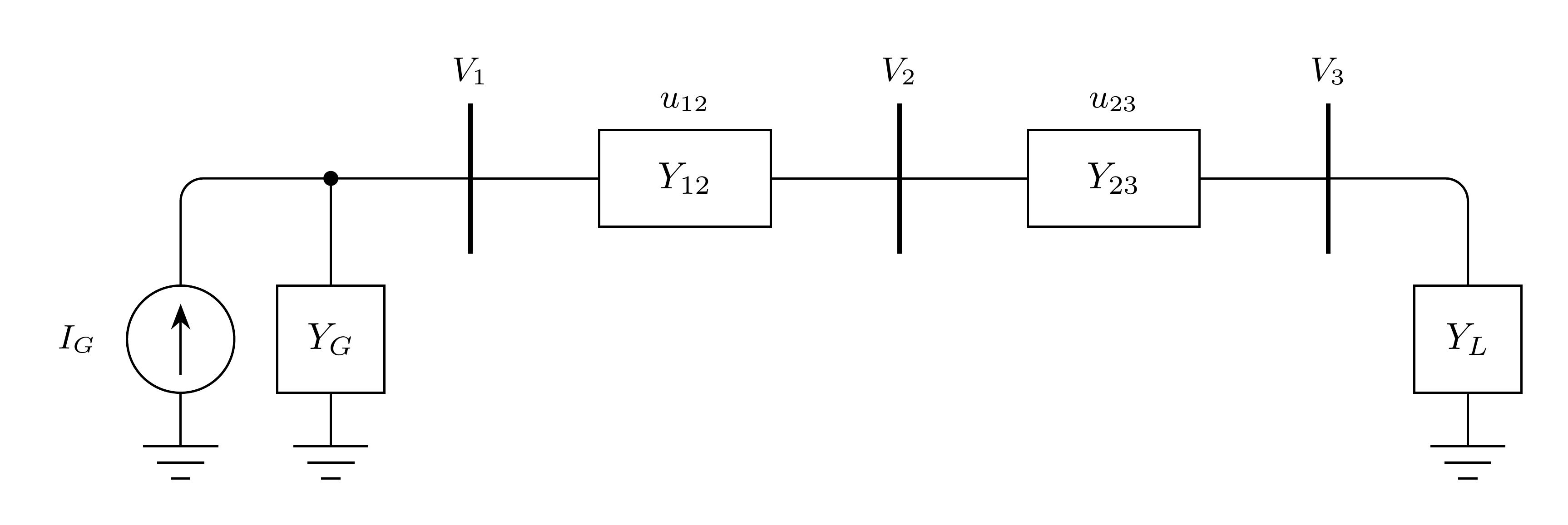
Since \(\mathbf{I} = (I_G, 0, 0)\) is constant, the Jacobian is the admittance matrix:

\[\begin{split}\begin{aligned} \mathbf{J} &= \dfrac{\partial \mathbf{F}}{\partial \mathbf{V}} = \mathbf{Y} \\ \mathbf{Y} &= u_{12} \begin{bmatrix} Y_{12} & -Y_{12} & 0 \\ -Y_{12} & Y_{12} & 0 \\ 0 & 0 & 0 \end{bmatrix} + u_{23} \begin{bmatrix} 0 & 0 & 0 \\ 0 & Y_{23} & -Y_{23} \\ 0 & -Y_{23} & Y_{23} \end{bmatrix} + \begin{bmatrix} Y_G & 0 & 0 \\ 0 & 0 & 0 \\ 0 & 0 & Y_L \end{bmatrix} \\ \det \mathbf{J} &= u_{12} u_{23} Y_{12} Y_{23} (Y_G + Y_L) + (u_{12} Y_{12} + u_{23} Y_{23}) Y_G Y_L \end{aligned}\end{split}\]

Scenario A.1: Isolated Bus

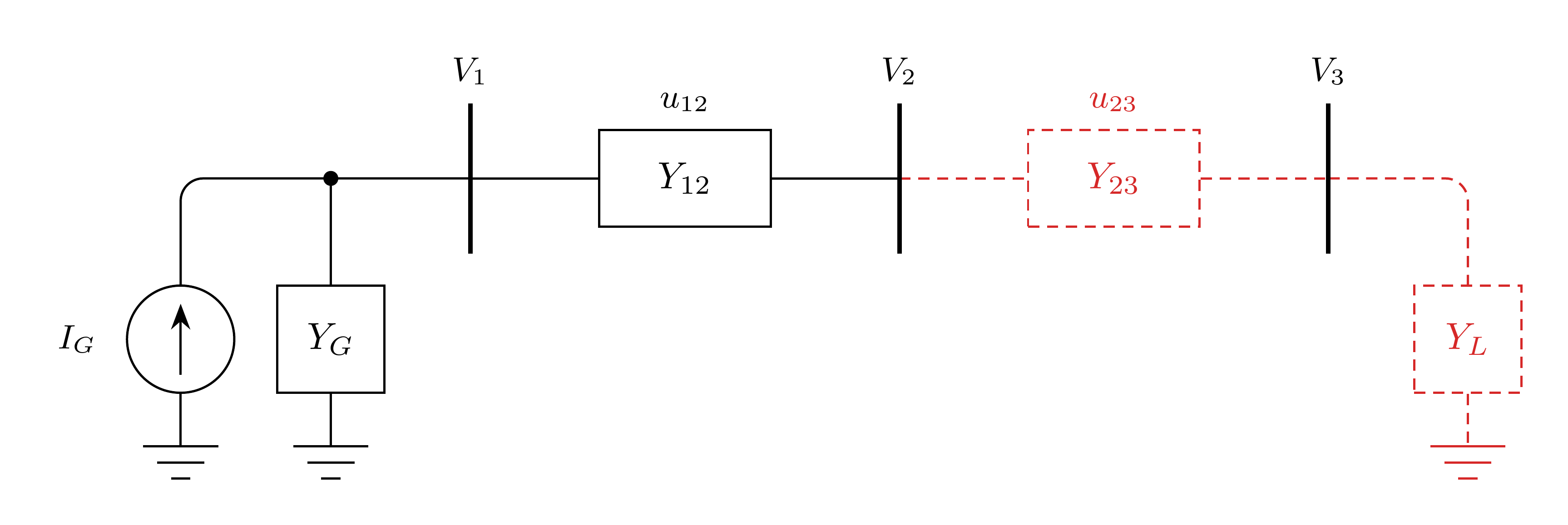
With \(u_{23} = 0\) and \(Y_L = 0\):

\[\begin{split}\begin{aligned} \mathbf{J} &= \begin{bmatrix} Y_G + Y_{12} & -Y_{12} & 0 \\ -Y_{12} & Y_{12} & 0 \\ 0 & 0 & 0 \end{bmatrix} \\ \det \mathbf{J} &= 0 \end{aligned}\end{split}\]

The bus 3 row is zero, so \(V_3\) is undetermined.

Scenario A.2: Floating Island

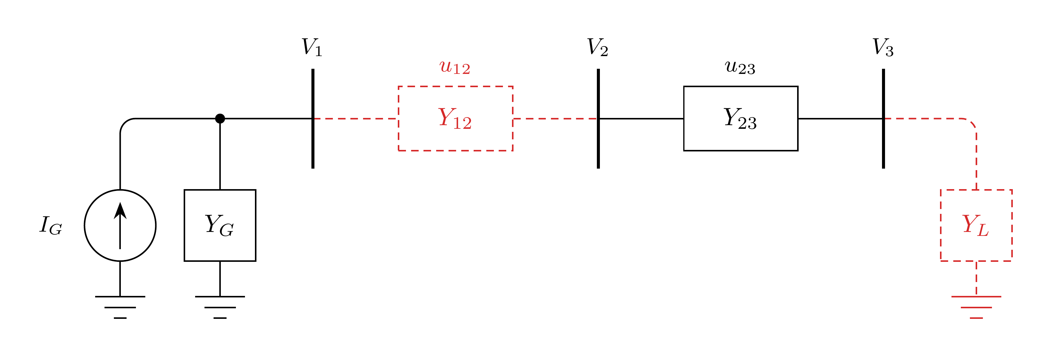
With \(u_{12} = 0\) and \(Y_L = 0\):

\[\begin{split}\begin{aligned} \mathbf{J} &= \begin{bmatrix} Y_G & 0 & 0 \\ 0 & Y_{23} & -Y_{23} \\ 0 & -Y_{23} & Y_{23} \end{bmatrix} \\ \det \mathbf{J} &= 0 \end{aligned}\end{split}\]

The island rows sum to zero, so \(V_2 = V_3\) is undetermined. (Edge case: Parallel branches whose taps or phase shifts disagree make the island nonsingular).

Scenario A.3: Grounded Island

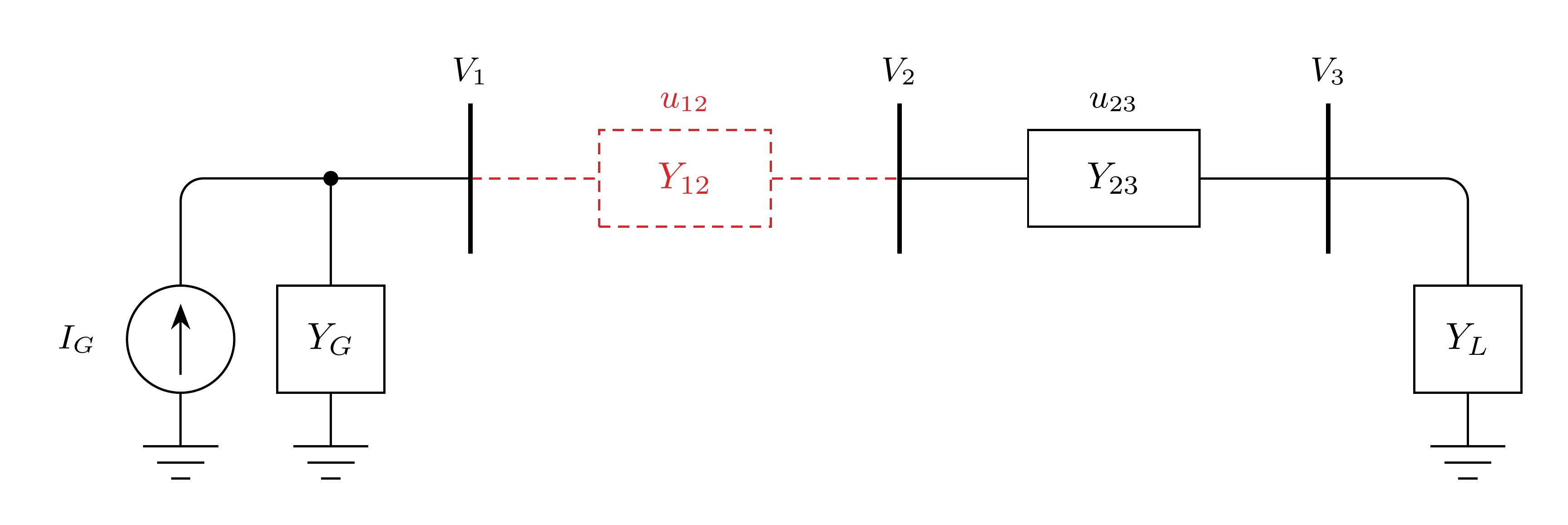
With \(u_{12} = 0\) and \(Y_L \neq 0\):

\[\begin{split}\begin{aligned} \mathbf{J} &= \begin{bmatrix} Y_G & 0 & 0 \\ 0 & Y_{23} & -Y_{23} \\ 0 & -Y_{23} & Y_{23} + Y_L \end{bmatrix} \\ \det \mathbf{J} &= Y_G Y_{23} Y_L \neq 0 \end{aligned}\end{split}\]

The load grounds the island. A fault or generator at bus 3 does the same.

Appendix B: Series Resonance

An outage can also make \(\mathbf{J}\) singular without creating an island. In the two-bus example below, bus 1 has a Norton generator with a capacitive \(Y_G\), as when a capacitor bank outweighs the generator’s own admittance, and the second circuit has status \(u\).

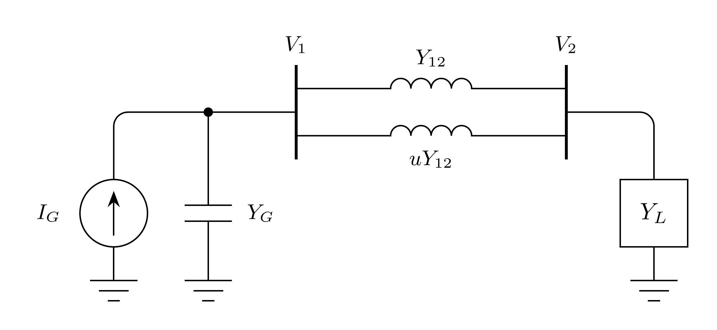
With \(Y_G = j\), \(Y_{12} = -j2\) per circuit, and \(Y_L = -j2\):

\[\begin{split}\begin{aligned} \mathbf{J} &= (1 + u) \begin{bmatrix} Y_{12} & -Y_{12} \\ -Y_{12} & Y_{12} \end{bmatrix} + \begin{bmatrix} Y_G & 0 \\ 0 & Y_L \end{bmatrix} \\ \det \mathbf{J} &= (1 + u) Y_{12} (Y_G + Y_L) + Y_G Y_L = -2u \end{aligned}\end{split}\]

Scenario B.1: Circuit Trip

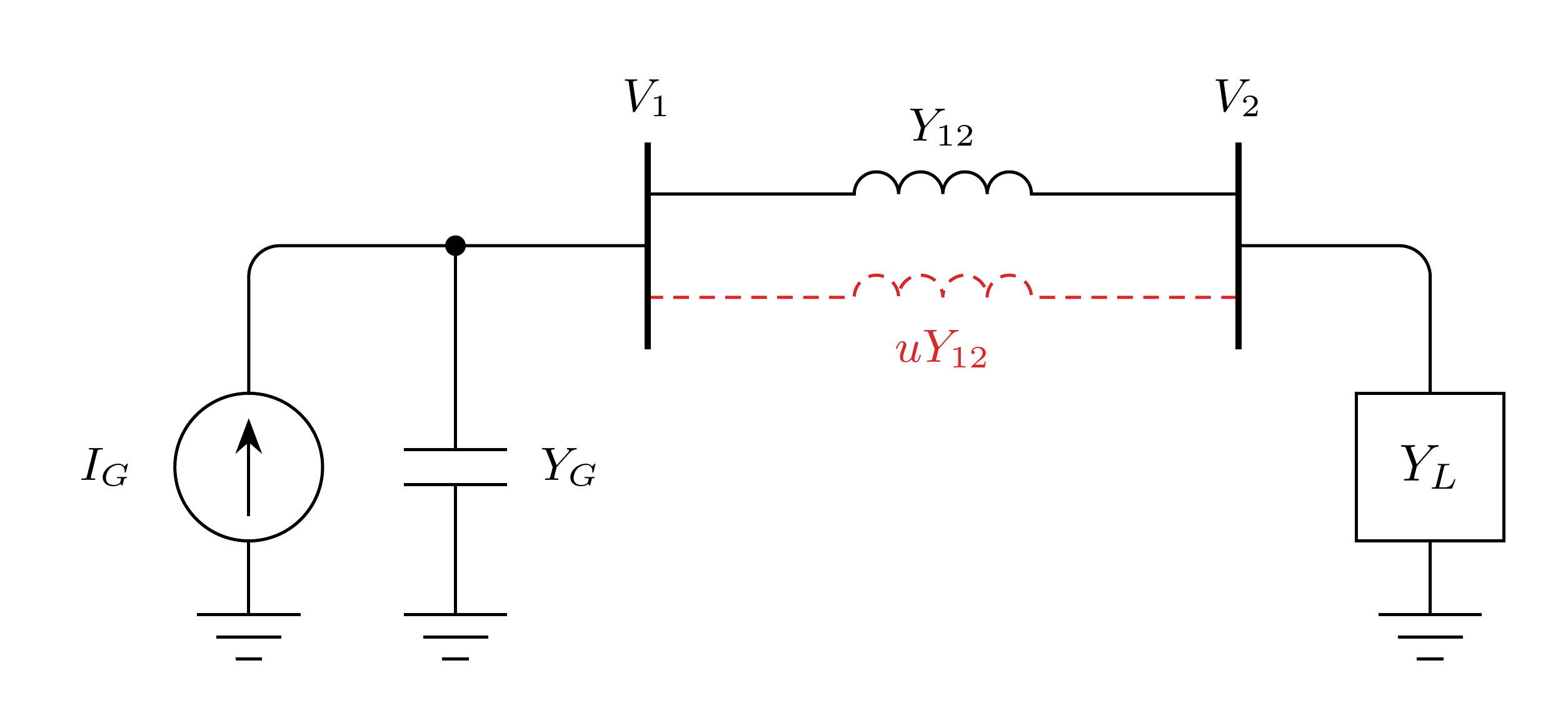
With \(u = 0\):

\[\begin{split}\begin{aligned} \mathbf{J} &= j \begin{bmatrix} -1 & 2 \\ 2 & -4 \end{bmatrix} \\ \det \mathbf{J} &= 0 \end{aligned}\end{split}\]

The network stays connected, but the loop impedance \(1/Y_G + 1/Y_{12} + 1/Y_L = -j + j0.5 + j0.5\) is zero, so the loop through ground is series resonant. Any resistance makes \(\det \mathbf{J} \neq 0\), but a nearly lossless loop still leaves \(\mathbf{J}\) ill-conditioned.